Data Structures, Algorithms, & Applications in Java
Suffix Trees
Copyright 1999 Sartaj Sahni
Have You Seen This String?
The Suffix Tree
Let's Find That Substring
Other Nifty Things You Can Do with a Suffix Tree
How to Build Your Very Own Suffix Tree
Exercises
References and Selected Readings
Have You Seen This String?
In the classical
substring search problem, we are given
a string
S and a pattern
P
and are to report whether or not the pattern
P
occurs in the string
S.
For example, the pattern
P = cat appears (twice)
in the string
S1 = The big cat ate the small catfish.,
but
does not appear in the string
S2 = Dogs for sale..
Researchers in the
human genome project
are constantly searching for substrings/patterns (we use the terms
substring and pattern interchangeably)
in a gene databank that contains tens of thousands of genes.
Each gene is represented as a sequence or string of letters drawn from
the alphabet
{A, C, G, T}. Although, most
of the strings in the databank are around
2000
letters long, some have tens of thousands of letters.
Because of the size of the gene databank and the frequency with which
substring searches are done, it is imperitive that we have as fast an
algorithm as possible to locate a given substring within the strings in the
databank.
We can search for a pattern
P
in a string
S,
using pattern matching algorithms that are described in standard
algorithm's texts.
The complexity of such a search is
O(|P| + |S|),
where
|P| denotes the length (i.e., number of
letters or digits) of
P.
This complexity looks pretty good when you consider that
the pattern
P could appear anywhere
in the string
S. Therefore,
we must
examine every letter/digit (we use the terms letter and
digit interchangeably) of the string before we can conclude that the
search pattern does not appear in the string. Further, before we can conclude
that the search pattern appears in the string, we must examine every
digit of the pattern. Hence, every
pattern search algorithm must take
time that is linear in the lengths of the pattern and the string being
searched.
When classical pattern matching
algorithms are used to search for several patterns
P1, P2, ..., Pk in the string
S,
O(|P1| + |P2| + ... + |Pk| + k|S|) time is taken
(because
O(|Pi| + |S|) time is taken to
seach for
Pi).
The suffix tree data structure that we are about to study reduces this
complexity to
O(|P1| + |P2| + ... + |Pk| + |S|).
Of this time,
O(|S|) time is spent setting up the suffix tree for
the string
S;
an individual pattern search takes only
O(|Pi|) time (after the suffix tree for
S has been built).
Therefore once the
suffix tree for
S has been created,
the time needed to search
for a pattern depends only on the length of the pattern.
The Suffix Tree
The
suffix tree for
S
is actually the
compressed trie
for the nonempty suffixes of the string
S.
Since a suffix tree is a compressed trie, we sometimes refer to the
tree as a trie and to its subtrees as subtries.
The (nonempty) suffixes of the string
S = peeper are
peeper, eeper, eper, per, er,
and
r.
Therefore, the suffix tree for the string
pepper
is the compressed trie that contains the elements (which are also the keys)
peeper, eeper, eper, per, er, and
r.
The alphabet for the string
peeper is
{e, p, r}. Therefore, the radix of the
compressed trie is
3.
If necessary, we may use the mapping
e -> 0, p -> 1, r -> 2, to
convert from the letters of the string to numbers.
This conversion is necessary only when we use a node structure in which
each node has an array of child pointers.
Figure 1 shows the compressed trie (with edge information) for the suffixes of
peeper.
This compressed trie is also the suffix tree for the string
peeper.
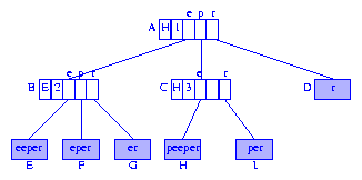
Figure 1 Compressed trie for the suffixes of peeper
Since the data in the information nodes
D-I
are the suffixes of
peeper, each information node
need retain only the start index of the suffix it contains.
When the letters in
peeper are indexed
from left to right beginning with the index
1,
the information nodes
D-I
need only retain the indexes
6, 2, 3, 5, 1, and
4,
respectively. Using the index stored in an information node, we can
access the suffix from the string
S.
Figure 2 shows the suffix tree of Figure 1 with each information node
containing a suffix index.
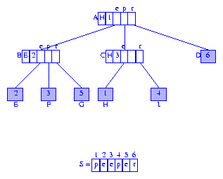
Figure 2 Modified compressed trie for the suffixes of peeper
The first component of each branch node is a reference to an element
in that subtrie. We may replace the element reference by the index of
the first digit of the referenced element. Figure 3 shows the resulting
compressed
trie.
We shall use this modified form as the representation for the suffix tree.

Figure 3 Suffix tree for peeper
When describing the search and construction algorithms for suffix trees,
it is easier to deal with a drawing of the suffix tree in which
the edges are labeled by the digits used in the move from a
branch node to a child node. The first digit of the label is the
digit used to determine which child is moved to, and the
remaining digits of the label give the digits that are skipped over.
Figure 4 shows the suffix tree of Figure 3 drawn in this manner.
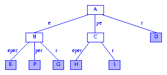
Figure 4 A more humane drawing of a suffix tree
In the more humane drawing of a suffix tree,
the labels on the edges
on any root to information node path
spell out the suffix represented by that information node.
When the digit number for the root is not
1,
the humane drawing of a suffix tree includes a head node with an
edge to the former root. This edge is labeled with the digits that
are skipped over.
The string
represented by a node of a suffix tree
is the string spelled by the labels on the path from the root to that node.
Node
A of Figure 4 represents the empty string
epsilon, node
C
represents the string
pe, and
node
F represents the string
eper.
Since the keys in a suffix tree are of different length, we must ensure that
no key is a proper prefix of another (see
Keys
With Different Length). Whenever the last digit of string
S appears only once in
S,
no suffix of
S can be a proper
prefix of another suffix of
S.
In the string
peeper, the
last digit is
r, and this digit appears only once.
Therefore, no suffix of
peeper is a proper prefix of another.
The last digit of
data is
a,
and this last digit appears twice in
data. Therefore,
data has two suffixes
ata and
a
that begin with
a. The suffix
a is a proper prefix of
the suffix
ata.
When the last digit of the string
S appears more than
once in
S we must append a new digit
(say
#) to the suffixes of
S
so that no suffix is a prefix of another. Optionally, we may append
the new digit to
S to get the string
S#, and then construct the suffix tree
for
S#. When this optional route is taken,
the suffix tree has one more suffix (
#) than
the suffix tree obtained by appending the symbol
# to the suffixes of
S.
Let's Find That Substring
But First, Some Terminology
Let
n = |S| denote the length (i.e., number of digits)
of the string whose suffix tree we are to build. We number the digits
of
S from left to right beginning with the number
1.
S[i] denotes the
ith digit of
S, and
suffix(i) denotes the suffix
S[i]...S[n] that begins at digit
i,
1 <= i <= n.
On With the Search
A fundamental observation used when searching for a
pattern
P in a string
S is that
P
appears in
S (i.e.,
P
is a substring of
S) iff
P is a prefix of some suffix of
S.
Suppose that
P = P[1]...P[k] =
S[i]...S[i+k-1]
.
Then,
P is a
prefix of
suffix(i).
Since
suffix(i) is in our compressed
trie (i.e., suffix tree), we
can search for
P by using the
strategy to search
for a key prefix in a compressed trie.
Let's search for the pattern
P = per
in the string
S = peeper. Imagine that we
have already constructed the suffix tree (Figure 4) for
peeper.
The search starts at the root node
A.
Since
P[1] =
p
, we follow the edge
whose label begins with the digit
p.
When following this edge, we compare the remaining digits
of the edge label with successive digits of
P.
Since these remaining label digits agree with the
pattern digits, we reach
the branch node
C. In getting to node
C, we have
used the first two digits of the pattern.
The third digit of the pattern is
r, and so,
from node
C we follow the edge whose label begins
with
r. Since this edge has no additional digits
in its label, no additional digit comparisons are done and we
reach the information node
I. At this time, the
digits in the pattern have been exhausted and we conclude that
the pattern is in the string. Since an information node is reached,
we conclude that
the pattern is actually a suffix of the string
peeper.
In the actual suffix tree representation (rather than in the humane drawing),
the information node
I contains the index
4 which tells us that the pattern
P = per begins at digit
4
of
peeper (i.e.,
P = suffix(4)).
Further, we can conclude that
per appears exactly once in
peeper; the search for a pattern that appears more than
once terminates at a branch node, not at an information node.
Now, let us search for the pattern
P = eeee.
Again, we start at the root. Since the first character of the pattern
is
e, we follow the edge whose label begins
with
e and reach the node
B.
The next digit of the pattern is also
e, and
so, from node
B we follow the edge whose label begins
with
e. In following this edge, we must compare
the remaining digits
per of the edge label with the
following digits
ee of the
pattern. We find a mismatch when the first pair
(p,e)
of digits are compared and we conclude that the pattern does not appear
in
peeper.
Suppose we are to search for the pattern
P = p.
From the root, we follow the edge whose label begins
with
p.
In following this edge, we compare
the remaining digits (only the digit
e remains)
of the edge label with the
following digits (there aren't any) of the
pattern. Since the pattern is exhausted while following this edge,
we conclude that the pattern is a prefix of all keys in the
subtrie rooted at node
C.
We can find all occurrences of the pattern by traversing the subtrie
rooted at
C and visiting the information
nodes in this subtrie. If we want the location of just one of the
occurrences of the pattern, we can use the index stored in the
first component of the branch node
C (see Figure 3).
When a pattern exhausts while following the edge to node
X, we say that node
X
has been reached; the search terminates at node
X.
When searching for the pattern
P = rope,
we use the first digit
r of
P
and reach the information node
D. Since the
the pattern has not been exhausted, we must check the
remaining digits of the pattern against those of the key in
D. This check reveals that the pattern is not a prefix
of the key in
D, and so the pattern does not
appear in
peeper.
The last search we are going to do is for the pattern
P = pepe. Starting at the root of Figure 4,
we move over the edge whose label begins with
p
and reach node
C. The next unexamined digit of the
search pattern is
p. So, from
node
C, we wish to follow the edge
whose label begins with
p. Since no edge
satisfies this requirement, we conclude that
pepe
does not appear in the string
peeper.
Other Nifty Things You Can Do with a Suffix Tree
Once we have set up the suffix tree for a string
S,
we can tell whether or not
S contains a pattern
P in
O(|P|) time.
This means that if we have a suffix tree for the text of Shakespeare's play
``Romeo and Juliet,'' we can determine whether or not the phrase
wherefore art thou appears in this play
with lightning speed. In fact, the time taken will be that needed to
compare up to
18 (the length of the
search pattern) letters/digits. The search time is independent of the
length of the play.
Other interesting things you can do at lightning speed are:
-
Find all occurrences of a pattern
P .
This is done by searching the suffix tree for P.
If P appears at least once, the
search terminates successfully
either at an information node or at a branch node. When the search terminates
at an information node, the pattern occurs exactly once. When we terminate
at a branch node X,
all places where the pattern occurs can be found by
visiting the information nodes in the subtrie rooted
at X.
This visiting can be done in time linear in the number of occurrences of the
pattern if we
- (a)
-
Link all of the information nodes in the suffix tree into a chain,
the linking is done in lexicographic order of the represented suffixes
(which also is the order in which the information nodes are encountered
in a left to right scan of the information nodes). The information nodes
of Figure 4 will be linked in the order
E, F, G, H, I, D.
- (b)
-
In each branch node, keep a reference to the first and last
information node in the subtrie of which that branch node is the root.
In Figure 4, nodes
A, B, and C
keep the pairs (E, D), (E, G),
and (H,I), respectively.
We use the pair (firstInformationNode, lastInformationNode)
to traverse the information node chain starting at
firstInformationNode and ending at
lastInformationNode. This traversal yields all
occurrences of patterns that begin with the string spelled
by the edge labels from the root to the branch node.
Notice that when (firstInformationNode, lastInformationNode)
pairs are kept in branch nodes, we can eliminate the branch node field that
keeps a reference to an information node in the subtrie (i.e., the field
element).
-
Find all strings that contain a pattern
P .
Suppose we have a collection S1, S2, ... Sk
of strings and we wish to report all strings that contain a query pattern
P. For example, the genome databank contains
tens of thousands of strings, and when a researcher submits a
query string, we are to report all databank strings
that contain the query string. To answer queries of this type efficiently,
we set up a compressed trie (we may call this a multiple
string suffix tree ) that contains the suffixes of the string
S1$S2$...$Sk#, where $ and
# are two different
digits that do not appear in any of the
strings S1, S2, ..., Sk.
In each node of the suffix tree, we keep a list
of all strings Si
that are the start point of a suffix represented by
an information node in that subtrie.
-
Find the longest substring of
S
that appears at least m > 1 times .
This query can be answered in O(|S|) time in the
following way:
- (a)
-
Traverse the suffix tree labeling the branch nodes with the sum of
the label lengths from the root and also with the number of information
nodes in the subtrie.
- (b)
-
Traverse the suffix tree visiting branch nodes
with information node count
>= m.
Determine the visited branch node with longest label length.
Note that step (a) needs to be done only once. Following this,
we can do step (b) for as many values of m
as is desired.
Also, note that when m = 2 we can avoid determining the
number of information nodes in subtries. In a compressed trie, every
subtrie rooted at a branch node has at least two information nodes in it.
-
Find the longest common substring of the strings
S and T .
This can be done in time O(|S| + |T|) as below:
- (a)
-
Construct a multiple string suffix tree for
S
and T (i.e., the suffix tree for
S$T#).
- (b)
-
Traverse the suffix tree to identify the branch node for
which the sum of the label lengths on the path from
the root is maximum and whose subtrie has at least one information
node that represents a suffix that begins in
S and at least one information
node that represents a suffix that begins in T.
Notice that the related problem to find the longest common subsequence
of S and T is solved
in O(|S| * |T|) time using dynamic programming
(see Exercise 15.22 of the text).
How to Build Your Very Own Suffix Tree
Three Observations
To aid in the construction of the suffix tree, we add a
longestProperSuffix field to each branch node.
The
longestProperSuffix field of a branch
node that represents the nonempty string
Y
points to the branch node for the longest proper
suffix of
Y
(this suffix is obtained by removing the first
digit from
Y).
The
longestProperSuffix field of the root is not used.
Figure 5 shows the suffix tree of Figure 4 with longest proper
suffix pointers (often, we refer to the longest proper
suffix pointer as simply the suffix pointer) included.
Longest proper suffix pointers are shown as red arrows.
Node
C represents the string
pe.
The longest proper suffix
e of
pe
is represented by node
B. Therefore, the
(longest proper) suffix pointer of
C points to node
B. The longest proper suffix of the string
e represented by node
B is the
empty string. Since the root node represents the empty string, the longest
proper suffix pointer of node
B points to the root node
A.
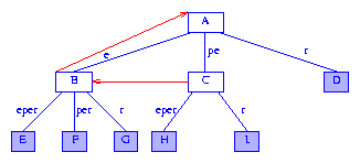
Figure 5 Suffix tree of Figure 4 augmented with suffix pointers
Observation 1
If the suffix tree for any string
S
has a branch node that represents the string
Y, then the tree also has a branch node that represents
the longest proper suffix
Z of
Y.
Proof
Let
P be the branch node for
Y.
Since
P is a branch node, there are at least
2 different digits
x and
y such that
S has
a suffix that begins with
Yx and another that
begins with
Yy.
Therefore,
S has
a suffix that begins with
Zx and another that
begins with
Zy.
Consequently, the suffix tree for
S
must have a branch node for
Z.
Observation 2
If the suffix tree for any string
S
has a branch node that represents the string
Y, then the tree also has a branch node for
each of the suffixes of
Y.
Proof
Follows from Observation 1.
Note that the suffix tree of Figure 5 has a branch node for
pe. Therefore, it also must have branch nodes
for the suffixes
e and
epsilon
of
pe.
The concepts of the
last branch node
and the
last branch index are useful
in describing the suffix tree construction algorithm.
The last branch node for suffix
suffix(i) is the
parent of the information node that represents
suffix(i). In Figure 5, the last branch nodes
for suffixes
1 through
6
are
C, B, B, C, B, and
A, respectively.
For any suffix
suffix(i), the last branch
index
lastBranchIndex(i) is the index of
the digit on which a branch is made at the last branch node
for
suffix(i).
In Figure 5,
lastBranchIndex(1) = 3
because
suffix(1) = peeper;
suffix(1) is represented by information node
H whose parent is node
C;
the branch at
C is made using the third digit
of
suffix(1); and the third digit of
suffix(1) is
S[3].
You may verify that
lastBranchIndex[1:6] =
[3, 3, 4, 6, 6, 6]
.
Observation 3
In the suffix tree for any string
S,
lastBranchIndex(i) <= lastBranchIndex(i+1),
1 <= i < n.
Proof
Left as an exercise.
Get Out That Hammer and Saw, and Start Building
To build your very own suffix tree, you must start with your very own string.
We shall use the string
R = ababbabbaabbabb
to illustrate the construction procedure. Since the last digit
b of
R appears more than
once, we append a new digit
# to
R
and build the suffix tree for
S = R# = ababbabbaabbabb#.
With an
n = 16 digit string
S,
you can imagine that this is going to be a rather long example.
However, when you are done with this example, you will
know everything you ever wanted to know about suffix tree construction.
Construction Strategy
The suffix tree construction algorithm starts with a root node that
represents the empty string. This node is a branch node.
At any time during the suffix tree construction process, exactly one
of the branch nodes of the suffix tree will be designated the
active node. This is the node from where the process
to insert the next suffix begins. Let activeLength be the
length of the string represented by the active node.
Initially,
the root is the active node and activeLength = 0.
Figure 6 shows the initial configuration, the active node is shown in green.

Figure 6 Initial configuration for suffix tree construction
As we proceed, we shall add branch and information nodes
to our tree. Newly added branch nodes will be colored
magenta, and newly added information nodes will be colored cyan.
Suffix pointers will be shown in red.
Suffixes are inserted into the tree in the order
suffix(1), suffix(2), ..., suffix(n).
The insertion of the suffixes in this order is accomplished by
scanning the string S from left to right.
Let tree(i) be the compressed trie
for the suffixes suffix(1), ..., suffix(i),
and let lastBranchIndex(j, i) be the last branch index
for suffix(j) in tree(i).
Let minDistance
be a lower bound on the distance (measured by number
of digits) from the active node to the last branch index of the
suffix that is to be inserted. Initially,
minDistance = 0 as
lastBranchIndex(1,1) = 1.
When inserting suffix(i), it will be the case that
lastBranchIndex(i,i) >= i + activeLength + minDistance.
To insert suffix(i+1) into
tree(i), we must do the following:
-
Determine
lastBranchIndex(i+1, i+1).
To do this, we begin at the current active node.
The first activeLength number of digits
of the new suffix (i.e., digits
S[i+1], S[i+2], ..., S[i + activeLength])
will be known to agree with the string represented
by the active node. So, to determine lastBranchIndex(i+1,i+1),
we examinine digits activeLength + 1,
activeLength + 2, ..., of the new suffix.
These digits are used to follow a path through tree(i)
beginning at the active node and terminating when
lastBranchIndex(i+1,i+1) has been determined.
Some efficiencies result from knowing that
lastBranchIndex(i+1,i+1) >= i + 1 + activeLength + minDistance.
-
If
tree(i) does not have
a branch node X
which represents the string
S[i]...S[lastBranchIndex(i+1,i+1)-1], then create
such a branch node X.
-
Add an information node for
suffix(i+1).
This information node is a child of the branch node X,
and the label on the edge from X to the
new information node is S[lastBranchIndex(i+1, i+1)]...S[n].
Back to the Example
We begin by inserting suffix(1) into
the tree tree(0) that is shown in Figure 6.
The root is the active node, activeLength = minDistance = 0.
The first digit of suffix(1) is S[1] = a.
No edge from the active node (i.e., the root) of tree(0)
has a label that begins with a
(in fact, at this time, the active node has no edge at all).
Therefore, lastBranchIndex(1,1) = 1. So,
we create an information node and an edge whose label is the entire
string. Figure 7 shows the result,
tree(1). The root remains the active node, and
activeLength and minDistance
are unchanged.
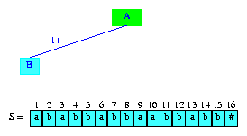
Figure 7 After the insertion of the suffix ababbabbaabbabb#
In our drawings, we shall show the
labels on edges that go to information nodes using the notation
i+, where i gives
the index, in S, where the label starts
and the + tells us that the label goes to
the end of the string.
Therefore, in Figure 7, the edge label 1+
denotes the string S[1]...S[n].
Figure 7 also shows the string S.
The newly inserted suffix is shown in cyan.
To insert the next suffix, suffix(2),
we again begin at the active node examining digits
activeLength + 1 = 1,
activeLength + 2 = 2, ..., of the new suffix.
Since, digit 1 of the new suffix is S[2] = b and
since the active node has no edge whose label
begins with S[2] = b,
lastBranchIndex(2,2) = 2. Therefore,
we create a new information node and an edge whose label is
2+. Figure 8 shows the resulting tree.
Once again, the root remains the active node and
activeLength and minDistance
are unchanged.
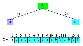
Figure 8 After the insertion of the suffix babbabbaabbabb#
Notice that the tree of Figure 8 is the compressed trie
tree(2)
for suffix(1) and
suffix(2).
The next suffix, suffix(3),
begins at S[3] = a. Since the
active node of tree(2) (i.e., the root)
has an edge whose label begins with a,
lastBranchIndex(3,3) > 3.
To determine
lastBranchIndex(3,3),
we must see more digits of suffix(3). In particular,
we need to see as many additional digits as are needed to distinguish between
suffix(1) and suffix(3).
We first compare
the second digit
S[4] = b
of the new suffix and the second digit S[2] = b
of the edge label 1+.
Since S[4] = S[2], we must do additional comparisons.
The next comparison is between the third digit S[5] = b
of the new suffix
and the third digit S[3] = a
of the edge label 1+.
Since these digits are different, lastBranchIndex(3,3)
is determined to be 5.
At this time, we update minDistance to have the
value 2.
Notice that, at this time, this is the max value possible
for minDistance
because
lastBranchIndex(3,3) = 5 = 3 + activeLength + minDistance.
To insert the new suffix,
suffix(3), we
split the edge of tree(2)
whose label is 1+ into two.
The first split edge has the label 1,2
and the label for the second split edge is 3+.
In between the two split edges, we place a branch node.
Additionally, we introduce an information node for the
newly inserted suffix.
Figure 9 shows the tree tree(3) that
results. The edge
label 1,2 is shown as the
digits S[1]S[2] = ab.
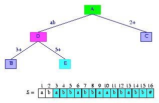
Figure 9 After the insertion of the suffix abbabbaabbabb#
The compressed trie tree(3)
is incomplete because we have yet to put in the
longest proper suffix pointer for the newly created
branch node D.
The longest suffix for this branch node is b, but
the branch node for b does not exist.
No need to panic, this branch node will be the next branch node
created by us.
The next suffix to insert is
suffix(4).
This suffix is the longest proper suffix of the most recently inserted
suffix, suffix(3). The insertion process
for the new suffix begins by updating the active node by following the
suffix pointer in the current active node. Since the root has
no suffix pointer, the active node is not updated. Therefore,
activeLength is unchanged also.
However, we must update minDistance to ensure
lastBranchIndex(4,4) >= 4 + activeLength + minDistance.
It is easy to see that
lastBranchIndex(i,i) <= lastBranchIndex(i+1,i+1)
for all i < n. Therefore,
lastBranchIndex(i+1,i+1) >= lastBranchIndex(i,i) >= i + activeLength + minDistance.
To ensure
lastBranchIndex(i+1,i+1) >= i + 1 + activeLength + minDistance,
we must reduce
minDistance by
1.
Since minDistance = 1,
we start at the active node (which is still the root) and move forward
following the path dictated by S[4]S[5]....
We do not compare the first minDistance
digits as we follow this path, because a match is
assured until we get to the point where
digit minDistance + 1 (i.e., S[5])
of the new suffix is to be compared.
Since the active node edge label that begins with
S[4] = b
is more than one digit long, we compare S[5] and the
second digit S[3] = a of this edge's label.
Since the two digits are different,
the edge is split in the same way we split the edge with label
1+. The first split edge has the label
2,2 = b, and the label on the second split
edge is 3+; in between the two
split edges, we place a new branch node F,
a new information node G is created for the
newly inserted suffix, this information node is connected
to the branch node F by an edge whose
label is 5+. Figure 10 shows the
resulting structure.
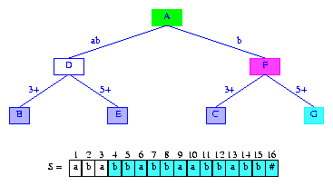
Figure 10 After the insertion of the suffix bbabbaabbabb#
We can now set the suffix pointer from the branch node
D that was created when
suffix(3) was inserted. This suffix
pointer has to go
to the newly created branch node F.
The longest proper suffix of the string b represented by
node F is the empty string. So, the suffix
pointer in node F is to point to the
root node.
Figure 11 shows the compressed trie with suffix pointers added.
This trie is tree(4).
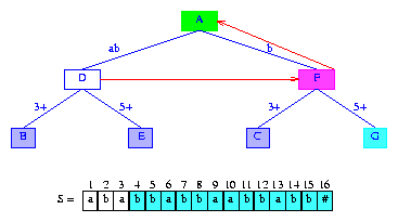
Figure 11 Trie of Figure 10 with suffix pointers added
The construction
of the suffix tree continues with an attempt to insert the next suffix
suffix(5).
Since suffix(5) is the longest proper suffix of
the most recently inserted suffix suffix(4),
we begin by following the suffix pointer in the active node. However,
the active node is presently the root and it has no suffix pointer. So,
the active node is unchanged. To preserve the desired
relationship among
lastBranchIndex, activeLength, minDistance,
and the index (5)
of the next suffix that is to be inserted,
we must reduce minDistance by one.
So, minDistance becomes zero.
Since activeLength = 0, we need to examine digits of
suffix(5) beginning with the first one
S[5].
The active node has an edge whose label begins with
S[5] = b.
We follow the edge with label b
comparing suffix digits and label digits.
Since all digits agree, we reach
node F. Node F
becomes the active node (whenever we encounter a branch node
during suffix digit examination, the active node is
updated to this encountered branch node) and
activeLength = 1.
We continue the comparison of
suffix digits using an edge from the current active node.
Since the next suffix digit to compare is
S[6] = a, we use an active node edge whose label
begins with a (in case such an
edge does not exist, lastBranchIndex for the
new suffix is activeLength + 1). This edge has the label
3+. The digit comparisons terminate
inside this label when digit S[10] = a
of the new suffix is compared with digit S[7] = b
of the edge label 3+.
Therefore, lastBranchIndex(5,5) = 10.
minDistance is set to its max possible value, which is
lastBranchIndex(5,5) - (index of suffix to be inserted) - activeLength = 10 - 5 - 1 = 4.
To insert suffix(5),
we split the
edge (F,C) that
is between nodes F and
C. The split takes place at digit
splitDigit = 5 of the label of
edge (F,C). Figure 12 shows the resulting tree.
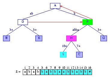
Figure 12 After the insertion of the suffix babbaabbabb#
Next, we insert suffix(6).
Since this suffix is the longest proper suffix of the last suffix
suffix(5) that we inserted,
we begin by following the suffix link in the active node. This gets us to
the tree root, which becomes the new active node.
activeLength becomes 0.
Notice that when we follow a suffix pointer, activeLength
reduces by 1; the value of
minDistance does not change because
lastBranchIndex(6,6) >= lastBranchIndex(5,5).
Therefore, we still have the desired relationship
lastBranchIndex(6,6) >= 6 + activeLength + minDistance.
From the new active node, we follow the edge whose label begins with
a. When an edge is followed, we do not compare
suffix and label digits. Since minDistance = 4,
we are assured that the first mismatch will occur five or more digits from here.
Since the label
ab that begins with a
is 2 digits long, we skip over
S[6] and S[7] of the
suffix, move to node D, make D
the active node, update activeLength to be
2 and minDistance to be
2,
and examine the label on the active node edge that begins
with S[8] = b. The label on this edge
is 5+. We omit the comparisons
with the first two digits of this label
because minDistance = 2 and
immediately compare the fifth digit S[10] = a of
suffix(6) with the third digit
S[7] = b of the edge label. Since these
are different, the edge is split at its third digit.
The new branch node that results
from the edge split is the node that the suffix pointer
of node H of Figure 12 is to point to.
Figure 13 shows the tree that results.
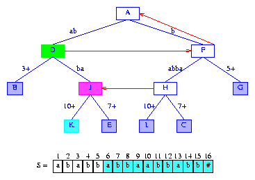
Figure 13 After the insertion of the suffix abbaabbabb#
Notice that following the last insertion, the active node is D,
activeLength = 2, and minDistance = 2.
Next, we insert suffix(7).
Since this suffix is the longest proper suffix of the
suffix just inserted, we can use
a short cut to do the insertion. The short cut
is to follow the suffix pointer in the current active node
D. By following this short cut, we skip
over a number of digits that is 1 less than
activeLength.
In our example, we
skip over 2 - 1 = 1 digit of
suffix(7).
The short cut guarantees a match between
the skipped over digits and the string represented by the node
that is moved to.
Node F becomes the new active node and
activeLength is reduced by 1.
Once again, minDistance is unchanged.
(You may verify that whenever a short cut is taken, leaving
minDistance unchanged satisfies the desired relationship
among lastBranchIndex, activeLength, minDistance,
and the index of the next suffix that is to be inserted.)
To insert suffix(7),
we use S[8] = b (recall that because of the
short cut we have taken to node F,
we must skip over activeLength = 1 digit of the suffix)
to determine the edge whose label is to be examined.
This gets us the label 5+. Again, since
minDistance = 2,
we are assured that
digits S[8] and S[9] of the
suffix match with the first two digits of the edge label
5+.
Since there is a mismatch at the third digit of the edge label, the
edge is split
at the third digit of its label. The suffix pointer of node
J is to point to the branch node that is placed between
the two parts of the edge just split. Figure 14 shows the result.
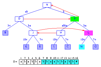
Figure 14 After the insertion of the suffix bbaabbabb#
Notice that following the last insertion, the active node is F,
activeLength = 1, and minDistance = 2.
If lastBranchIndex(7,7) had turned out to be greater
than 10, we would increase minDistance
to lastBranchIndex(7,7) - 7 - activeLength.
To insert suffix(8), we first take
the short cut from the current active node F
to the root. The root becomes the new active node, activeLength
is reduced by 1 and
minDistance is unchanged.
We start the insert process at the new active node.
Since minDistance = 2, we have to move at least
3 digits down from the active node.
The active node edge whose label begins with S[8] = b
has the label b.
Since minDistance = 2,
we must follow edge labels until we have skipped
2 digits. Consequently, we move to
node F. Node F
becomes the active node, minDistance
is reduced by the length 1 of the label on the edge
(A,F) and becomes
1, activeLength is increased
by the length of the label on the edge
(A,F) and becomes
1,
and we follow the edge (F,H)
whose label
begins with S[9] = a.
This edge is to be split at the second digit of its edge label.
The suffix pointer of
L is to point to the
branch node that will be inserted between the two edges created
when edge (F,H) is split.
Figure 15 shows the result.
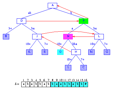
Figure 15 After the insertion of the suffix baabbabb#
The next suffix to insert is suffix(9).
From the active node F,
we follow the suffix pointer to node A, which
becomes the new active node.
activeLength is reduced by 1
to zero, and minDistance is unchanged
at 1.
The active node edge whose label begins with S[9] = a
has the label ab.
Since minDistance = 1,
we compare the second digit of suffix(9)
and the second digit of the edge label. Since these two digits are different,
the edge (A,D) is split at the
second digit of its label.
Further the suffix pointer of the branch node M
that was created when the last suffix was inserted into the trie, is to point to
the branch node that will be placed between nodes A
and D. Finally, since the newly created branch node
represents a string whose length is one, its suffix pointer
is to point to the root.
Figure 16 shows the result.
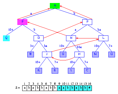
Figure 16 After the insertion of the suffix aabbabb#
As you can see, creating a suffix trie can be quite tiring.
Let's continue though, we have, so far,
inserted only the first 9
suffixes into our suffix tree.
For the next suffix, suffix(10),
we begin with the root A as the active node.
We would normally follow the suffix pointer in the active node
to get to the new active node from which the insert process is to start.
However, the root has no suffix pointer. Instead, we reduce
minDistance by one. The new value of
minDistance is zero.
The insertion process begins by
examining the active node edge (if any) whose label begins with
the first digit
S[10] = a of suffix(10).
Since the active node has an edge whose label begins with
a, additional digits are examined to determine
lastBranchIndex(10,10).
We follow a search path from the active node.
This path is determined by the digits of suffix(10).
Following this path, we reach node J. By examining
the label on the edge (J,E), we determine that
lastBranchIndex(10,10) = 16.
Node J
becomes the active node,
activeLength = 4,
and minDistance = 2.
When suffix[10] is inserted,
the edge (J,E) splits. The split is at the
third digit of this edge's label.
Figure 17 shows the tree after the new suffix is inserted.
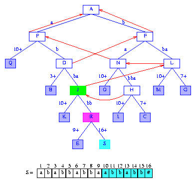
Figure 17 After the insertion of the suffix abbabb#
To insert the next suffix, suffix(11),
we first take a short cut by following
the suffix pointer at the
active node. This pointer gets us to node L, which
becomes the new active node. At this time, activeLength
is reduced by one and becomes 3.
Next, we need to move forward
from L by a number of digits greater than
minDistance = 2.
Since digit activeLength + 1 of suffix(11)
is S[14] = b we follow the b
edge of L. We omit comparing the first
minDistance digits of this edge's label.
The first comparison made is between
S[16] = # (digit of suffix) and
S[7 + 2] = a (digit of edge label).
Since these two digits are different,
edge (L,G) is to be split.
Splitting this edge (at its third digit) and setting the suffix pointer
from the most recently created branch node R gives
us the tree of Figure 18.
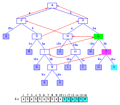
Figure 18 After the insertion of the suffix bbabb#
To insert the next suffix, suffix(12),
we first take the short cut from the current
active node L
to the node N. Node N becomes the
new active node, and we begin comparing
minDistance + 1 = 3
digits down from node N.
Edge (N,H) is split. Figure 19 shows the tree
after this edge has been split and after the suffix pointer from the most
recently created
branch node T
has been set.
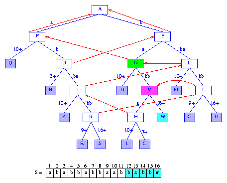
Figure 19 After the insertion of the suffix babb#
When inserting suffix(13),
we follow the short cut from the active node N
to the branch node P. Node P
becomes the active node and we are to move down the tree by at least
minDistance + 1 = 3 digits.
The active node edge whose label begins with
S[14] = b is used first.
We reach node
D, which becomes
the active node, and minDistance
becomes 1. At node D, we
use the edge
whose label begins with S[15] = b. Since the label
on this edge
is two digits long, and since the second digit of this label
differs from S[16],
this edge is to split. Figure 20
shows the tree after the edge is split and the suffix pointer from
node V is set.
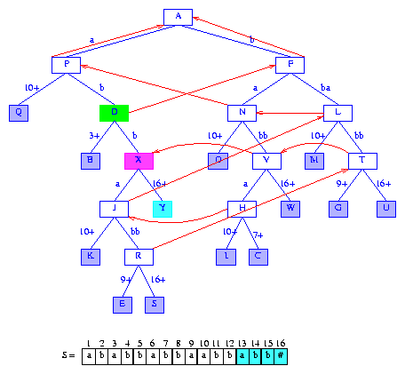
Figure 20 After the insertion of the suffix abb#
To insert suffix(14),
we take the short cut from the current active node D
to the branch node F. Node F
becomes the active node. From node F, we must move
down by at least minDistance + 1 = 2 digits.
We use the edge whose label begins with S[15] = b
(S[15] is used because it is activeLength = 1 digits from the start of
suffix(14)).
The split takes place at the second digit of edge
(F,L)'s label. Figure 21 shows the new tree.
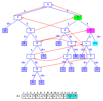
Figure 21 After the insertion of the suffix bb#
The next suffix to insert begins at S[15] = b.
We take the short cut from the current active node F,
to the root. The root is made the current active node
and then we move down by minDistance + 1 = 2
digits.
We follow the active node edge whose label begins with b
and reach node F.
A new information node is added to F.
The suffix pointer for the
last branch node Z is set
to point to the current active node F,
and the root becomes the new active node.
Figure 22 shows the new tree.
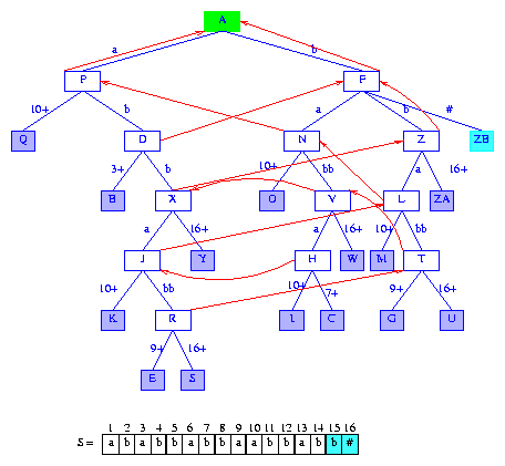
Figure 22 After the insertion of the suffix b#
Don't despair, only one suffix remains. Since no suffix is a proper
prefix of another suffix, we are assured that the root has no edge
whose label begins with the last digit of the string S.
We simply insert an information node as a child of the root. The
label for the edge to this new information node is the last digit of
the string. Figure 23 shows the complete suffix tree for
the string S = ababbabbaabbabb#.
The suffix pointers are not shown as they are no longer needed;
the space occupied by these pointers may be freed.
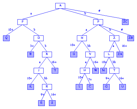
Figure 23 Suffix tree for ababbabbaabbabb#
Complexity Analysis
Let r denote the number of different digits
in the string S whose
suffix tree is to be built (r is the alphabet
size), and let n be the number of digits
(and hence the number of suffixes) of the string S.
To insert suffix(i), we
- (a)
-
Follow
a suffix pointer in the active node
(unless the active node is the root).
- (b)
-
Then move down the existing suffix tree
until
minDistance digits have been crossed.
- (c)
-
Then compare some number of suffix digits with edge label digits
until
lastBranchIndex(i,i)
is determined.
- (d)
-
Finally insert a new information node and possibly also
a branch node.
The total time spent in part (a) (over all n inserts) is
O(n).
When moving down the suffix tree in part (b), no digit comparisons are made.
Each move to a branch node at the next level takes O(1)
time. Also, each such move reduces the value of
minDistance by at least one. Since
minDistance
is zero initially and never becomes less than zero, the total time
spent in part (b) is O(n + total amount by which minDistance
is increased over all n inserts).
In part (c), O(1) time is spent determining whether
lastBranchIndex(i,i) = i + activeLength + minDistance.
This is the case iff
minDistance = 0
or
the digit x at position
activeLength + minDistance + 1
of suffix(i) is not the same
as the digit in position minDistance + 1
of the label on the appropriate edge of the active node.
When
lastBranchIndex(i,i) != i + activeLength + minDistance,
lastBranchIndex(i,i) > i + activeLength + minDistance and
the value of
lastBranchIndex(i,i) is determined by making
a sequence of comparisons between suffix digits and edge label digits (possibly
involving moves downwards to new branch nodes). For each such comparison
that is made, minDistance is increased by
1. This is the only circumstance under
which minDistance increases in the algorithm.
So, the total time
spent in part (c) is O(n + total amount by which minDistance
is increased over all n inserts).
Since each unit increase in the value of minDistance
is the result of an equal compare between a digit at a new
position (i.e., a position from which such a compare
has not been made previously) of the string S
and an edge label digit,
the total amount by which minDistance
is increased over all n inserts is
O(n).
Part (d) takes
O(r) time per insert, because we need to initialize
the O(r) fields of the branch node that may be created.
The total time for part (d) is, therefore, O(nr).
So, the total time taken to
build the suffix tree is O(nr).
Under the assumption that the alphabet size r
is constant, the complexity of
our suffix tree generation algorithm becomes O(n).
The use of branch nodes with as many children fields as the alphabet size
is recommended only when the alphabet size is small.
When the alphabet size is large (and it may be as large as
n, making the above algorithm an
O(n2) algorithm),
the use of a
hash table results in an expected time complexity of
O(n). The space complexity changes
from O(nr) to O(n).
A divide-and-conquer algorithm that has a time and space
complexity of O(n) (even when the alphabet
size is O(n)) is developed in
Optimal suffix tree construction with large alphabets.
Exercises
-
Draw the suffix tree for
S = ababab#.
-
Draw the suffix tree for
S = aaaaaa#.
-
Draw the multiple string suffix tree for
S1 = abba, S2 = bbbb, and s3
= aaaa.
-
Prove Observation 3.
-
Draw the trees
tree(i), 1 < = i < = |S|
for S = bbbbaaaabbabbaa#.
Show the active node in each tree.
Also, show the longest proper suffix pointers.
-
Draw the trees
tree(i), 1 < = i < = |S|
for S = aaaaaaaaaaaa#.
Show the active node in each tree.
Also, show the longest proper suffix pointers.
-
Develop the class
SuffixTree.
Your class should include a method to create the suffix tree for a
given string as well as a method to search a suffix tree for a given
pattern. Test the correctness of your methods.
-
Explain how you can obtain the multiple string suffix tree
for
S1, ..., Sk from that for
S1, ..., S(k-1).
What is the time complexity of your proposed method?
References and Selected Readings
You can learn more about the genome project and
genomic applications of pattern matching from the following Web sites:
-
NIH's Web site for the human genome project
-
Department of Energy's Web site for the human genomics project
-
Biocomputing Hypertext Coursebook.
Linear time algorithms to search for a single pattern in a given string
can be found in most algorithm's texts. See, for example, the texts:
-
Computer Algorithms , by E. Horowitz, S. Sahni, and
S. Rajasekeran, Computer Science Press, New York, 1998.
-
Introduction to Algorithms , by T. Cormen, C. Leiserson, and
R. Rivest, McGraw-Hill Book Company, New York, 1992.
For more on suffix tree construction, see the papers:
-
``A space economical suffix tree construction algorithm,'' by
E. McCreight, Journal of the ACM ,
23, 2, 1976, 262-272.
-
``On-line construction of suffix trees,'' by E. Ukkonen,
Algorithmica , 14, 3, 1995, 249-260.
-
Fast string searching with suffix trees,'' by M. Nelson,
Dr. Dobb's Journal , August 1996.
-
Optimal suffix tree construction with large alphabets, by M. Farach,
IEEE Symposium on the Foundations of Computer Science , 1997.
You can download C++ code to construct a suffix tree from
http://www.ddj.com/ftp/1996/1996.08/suffix.zip. This code, developed
by M. Nelson, is described in paper 3 above.